Probability Distribution Calculator
Use our probability distribution calculator to find the mean, standard deviation, and variance of a distribution by entering each value x and its probability P(x) below. Plus, see the steps to solve below.
Results:
| Mean (μ): | |
|---|---|
| Standard Deviation (σ): | |
| Variance (σ²): |
How to Find the Mean:
To find the mean for a distribution, use the following formula:
μ = ∑x · p(x)
The mean for a distribution is equal to the sum of each value times the probability of the value occurring.
To find the mean, multiply each value times each probability, then add them all together.
How to Find the Variance:
To find the variance for a distribution, use the following formula:
σ² = ∑x² · p(x) - μ²
The variance for a distribution is equal to the sum of each value squared times the probability of the value occurring, minus the mean squared.
How to Find the Standard Deviation:
The standard deviation is equal to the square root of the variance:
So, to find the standard deviation, take the square root of the variance.
On this page:
- Probability Distribution Calculator
- What is a Probability Distribution?
- Normal Probability Distribution
- Discrete Probability Distribution
- Continuous Probability Distribution
- Binomial Probability Distribution
- Poisson Probability Distribution
- How to Find the Mean of a Probability Distribution
- How to Find the Variance of a Probability Distribution
- How to Find the Standard Deviation of a Probability Distribution
- References

Joe is the creator of Inch Calculator and has over 20 years of experience in engineering and construction. He holds several degrees and certifications.

Brian specializes in political science and statistics with several advanced degrees from Harvard.
What is a Probability Distribution?
In statistics, a probability distribution is a function that describes the probability of all events associated with a random variable.[1] For example, the flip of a fair coin has a probability distribution that gives equal probability to heads or tails. The likelihood of getting a particular value varies based on the underlying distribution.
Normal Probability Distribution
One of the most frequently arising probability distributions is a normal distribution. If you analyze the totals of a series of similar random events (for example, how many heads out of many flips from the same coin), that total will at least approximately follow a normal distribution.
Since arithmetic means are calculated using sum totals, it also follows that average outcomes will also often follow a normal distribution. The normal distribution has a familiar shape of a perfect bell curve when graphed. The results of a coin flip follow a discrete probability distribution, since a coin flip can only take one of several possible values.
The normal distribution is an example of a continuous probability distribution, which describes events that can take a range of numerical values, for example, temperature. Note that the range of the normal distribution is not bounded, meaning it assigns some probability to events that are very unlikely (daily temperatures above boiling) or impossible (temperatures below absolute zero).
Even so, the normal distribution often still describes well such cases because, depending on the distribution’s center and spread, it can assign almost zero chances to cases that are extremely far-fetched or even impossible.
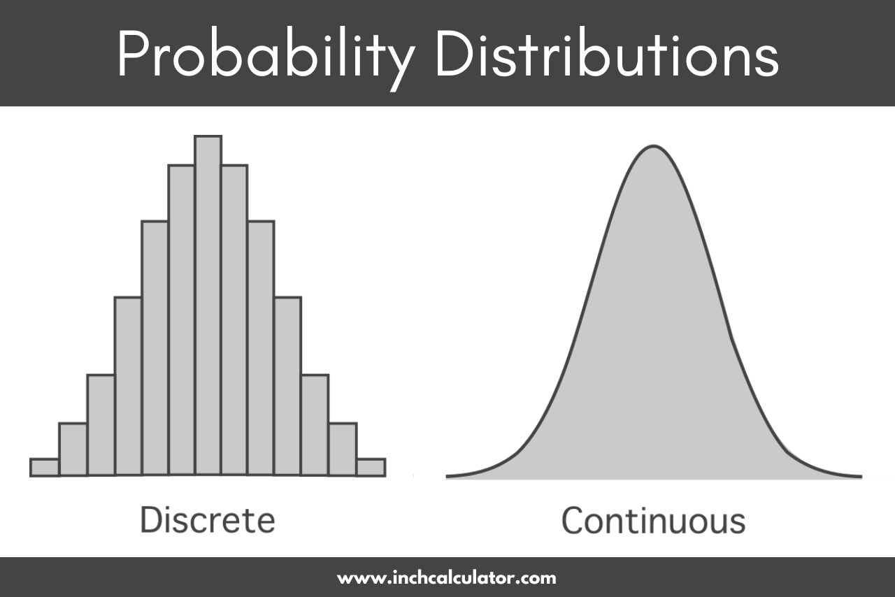
Discrete Probability Distribution
As mentioned above, a discrete probability distribution is a distribution over discrete, or countable, outcomes. In a discrete probability distribution, the probability of a value is defined by its probability mass function (PMF).
This means that each event has a particular numerical probability associated with it; for example, heads has a probability of 0.5 if the coin is fair. All distributions over a finite set of outcomes are discrete, however not all discrete distributions are finite. For example, suppose you wanted to flip a coin until it lands on heads.
The number of times the coin lands on tails will follow a negative binomial distribution, and there is at least some chance that you would have three tails, ten tails, or indeed a thousand or more tails before the coin lands on heads. A distribution is discrete because it assigns a particular number to a particular outcome, but the distribution can do that provided there is a countable number of outcomes.
Continuous Probability Distribution
For outcomes that are continuous, associating a numerical probability with a particular outcome is impossible. What are the chances that the temperature is exactly 72 degrees at a particular day and time? Effectively zero, the temperature if accurately measures is likely to be closer to 72.1 or 72.01.
To get around these difficulties, it makes sense to define probabilities for continuous distributions through its probability density function (PDF). The “term” density in the name of this function comes from an analogy to physics, as volume times density gives mass. Similarly, combining information about the range of values you are interested in with the probability density function gives a probability mass.
Doing so, you can assign numerical probability to events like the temperature being between 71.5 and 72.49 degrees. Chi-squared distributions, T distributions, F distributions, and Weibull distributions are other examples of continuous probability distributions.
Binomial Probability Distribution
So far we have had occasion to mention the number of heads from a series of coin flips. This is an instance of a more general discrete distribution called the binomial probability distribution. In a binomial distribution, the outcomes are binary, or yes/no outcomes, and the number of successes in n trials of the experiment are reflected in the distribution.
Importantly, the binomial distribution can describe situations where the yes/no outcomes are not equally likely.
Poisson Probability Distribution
A Poisson probability distribution is another example of a discrete distribution. It is often used in situations where you count the number of some outcomes in a particular interval of time, where the arrival of one outcome does not make the next outcome more or less likely.
For instance, you might show a distribution showing the number of cars that drive past your home every hour. The Poisson distribution is another example of discrete but not finite distributions.
You can use our probability or Bayes’ theorem calculators to find the likelihood of an event.
How to Find the Mean of a Probability Distribution
One characteristic of a probability distribution is the mean, or more frequently the average (although this is imprecise because there are many different kinds of averages). The mean is also sometimes called its expected value. You can find the mean for a probability distribution using the following formula:
μ = ∑x · p(x)
Thus, the population mean for a probability distribution is equal to the sum of each value x times the probability of the value occurring p(x).
Put more simply, you can find the mean by multiplying each value times its probability of success, then add them all together.
For example, let’s find the mean for the following probability distribution:
| x | 1 | 2 | 3 | 4 | 5 |
|---|---|---|---|---|---|
| p(x) | 0.2 | 0.25 | 0.4 | 0.12 | 0.03 |
Start by substituting each value and probability into the mean equation.
μ = (1 · 0.2) + (2 · 0.25) + (3 · 0.4) + (4 · 0.12) + (5 · 0.03)
μ = 0.2 + 0.5 + 1.2 + 0.48 + 0.15
μ = 2.53
So, the mean μ for this probability distribution is equal to 2.53.
The mean is frequently also a key parameter that allows you to use the probability distribution to calculate the probability of particular events. In the case of the normal distribution, the mean defines the center of the distribution.
How to Find the Variance of a Probability Distribution
Another characteristic of a probability distribution is the variance, which is a measure of the dispersion or “spread” within the data. Variance is represented as σ² (pronounced sigma-squared).
You can find the variance using the following formula:
σ² = ∑x² · p(x) – μ²
The variance for a probability distribution is equal to the sum of each value x squared times the probability of the value occurring p(x), minus the mean μ squared.
For example, let’s find the variance for the following probability distribution:
| x | 5 | 10 | 15 | 20 |
|---|---|---|---|---|
| p(x) | 0.1 | 0.35 | 0.25 | 0.3 |
Start by solving the first portion of the formula, which is the sum of each value squared multiplied by the probability of it occurring.
∑x² · p(x) = (5² · 0.1) + (10² · 0.35) + (15² · 0.25) + (20² · 0.3)
∑x² · p(x) = (25 · 0.1) + (100 · 0.35) + (225 · 0.25) + (400 · 0.3)
∑x² · p(x) = 2.5 + 35 + 56.25 + 120
∑x² · p(x) = 213.75
Then, subtract the mean μ squared from this result. Using the formula above, the mean for this distribution is 13.75.
σ² = 213.75 – 13.75²
σ² = 213.75 – 189.0625
σ² = 24.6875
The variance for this distribution is equal to 24.6875.
Similar to the mean, the variance is also frequently a key parameter that allows you to define the probability of various events according to a probability distribution. For example, the normal distribution is specified using both the mean and variance.
How to Find the Standard Deviation of a Probability Distribution
Closely related to the variance of a probability distribution is its standard deviation. In some cases, it may be easier to think about standard deviation as a measure of spread than variance.
It refers to the expected absolute difference between a particular observation and the mean observation. If the difference between a typical observation and the mean observation is small, i.e. the standard deviation is small, the data is tightly packed and the distribution is not widely spread.
Conversely, if the standard deviation is large, observations are typically far from the mean. The standard deviation is represented by the Greek letter sigma σ, and it’s equal to the square root of the variance.
So, to find the standard deviation, find the variance using the steps above, then take the square root.
σ = √σ²
All normal distributions are related to the so-called standard normal distribution, which has mean 0 and standard deviation (or equivalently) variance of 1. That means, for any set of events coming from a normal distribution, you can demean (i.e. substract the mean) and rescale (i.e. divide by the standard deviation) the observations, and the result will come from a standard normal distribution.
This fact is widely used in statistics to calculate quantities such as z-scores, p-values, and other indicators of statistical significance.
Similar Statistics Calculators
References
- Blitzstein, J., and Hwang, J., Introduction to Probability, 95. https://probabilitybook.net