Binomial Distribution Calculator
Enter the probability of success for a single trial, the number of trials, and the number of successes to calculate the binomial and cumulative probabilities of getting successful events.
Results: Probabilities
| P(X = x): | |
|---|---|
| P(X < x): | |
| P(X ≤ x): | |
| P(X > x): | |
| P(X ≥ x): |
On this page:

Joe is the creator of Inch Calculator and has over 20 years of experience in engineering and construction. He holds several degrees and certifications.


How to Calculate a Binomial Distribution
In statistics, a binomial distribution is a probability distribution of the number of successes in a sequence of independent experiments or trials. The result of each experiment must be dichotomous, which means the result must be a yes/no, success/fail, heads/tails, true/false, or similar outcome.
Unlike a normal distribution, a binomial distribution is a probability distribution for a discrete variable, while a normal distribution describes a continuous variable. Binomial distributions can be skewed or symmetrical, while a normal distribution is always symmetrical.
Each experiment in a sequence is referred to as a trial, or more specifically, a Bernoulli trial. The sequence is sometimes referred to as a Bernoulli process, named for mathematician Jacob Bernoulli.
The binomial distribution describes the likelihood of possible outcomes from a set of trials.
To help better understand the binomial distribution, let’s use the example of recording coin flips. Let’s say we ran a sequence of 100 coin flips and measured the number of times it landed on heads. If we repeated this sequence of one hundred flips 20,000 times and plotted the number of heads in each sequence, we might see a distribution like this one.
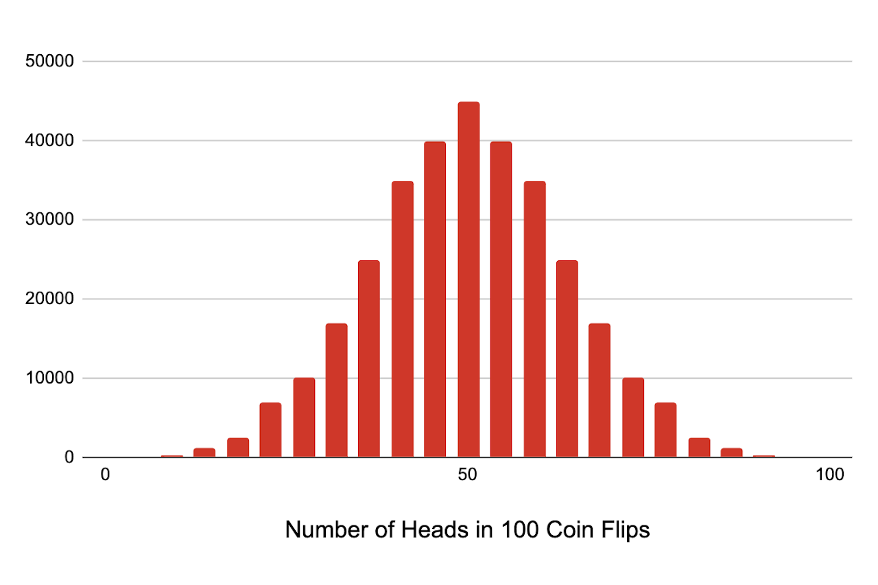
In this sequence, the number of trials n is 100, representing the 100 coin flips. The number of successes x is the number of times in the sequence that the coin landed on heads. The probability p is 0.5 since there is a 50% chance of landing on heads.
How to Calculate a Binomial Probability
A binomial probability is the probability of getting exactly x successes in a sequence of n trials, where the probability p of success in each trial is the same. Each trial must be independent, meaning that the results of one trial do not influence the probability that the next trial will be successful.
There are a few ways to calculate a binomial probability. The first method is to use a formula, and the second is to refer to a binomial probability distribution chart.
Binomial Probability Formula
You can calculate the binomial probability using the binomial probability mass function:[1]
The binomial probability mass function (PMF) states that the probability of x successes in a sequence of n independent trials with a probability of success in a single trial p is equal to the number of possible combinations of success times p to the power of x times 1 minus p to the power of n minus x.
You may also see the probability mass function referred to as the binomial probability density function (PDF). But, because a binomial distribution is a distribution of a discrete variable rather than a continuous variable, it is technically a mass function, not a density function.
You can calculate the number of possible combinations using our combinations calculator. The number of combinations can also be found using the formula:
The number of combinations is equal to the number of events or trials n factorial divided by the number of successes x factorial times n minus x factorial. Our factorial calculator might be useful for this calculation.

Binomial Probability Distribution Table
The binomial distribution table below shows the probability of getting x successes in a sample of n trials, with a probability of success in each trial p.
| p | ||||||||||||
| x | 0.05 | 0.10 | 0.20 | 0.30 | 0.40 | 0.50 | 0.60 | 0.70 | 0.80 | 0.90 | 0.95 | |
| n = 1 | 0 | 0.950 | 0.900 | 0.800 | 0.700 | 0.600 | 0.500 | 0.400 | 0.300 | 0.200 | 0.100 | 0.050 |
| 1 | 0.050 | 0.100 | 0.200 | 0.300 | 0.400 | 0.500 | 0.600 | 0.700 | 0.800 | 0.900 | 0.950 | |
| n = 2 | 0 | 0.903 | 0.810 | 0.640 | 0.490 | 0.360 | 0.250 | 0.160 | 0.090 | 0.040 | 0.010 | 0.003 |
| 1 | 0.095 | 0.180 | 0.320 | 0.420 | 0.480 | 0.500 | 0.480 | 0.420 | 0.320 | 0.180 | 0.095 | |
| 2 | 0.003 | 0.010 | 0.040 | 0.090 | 0.160 | 0.250 | 0.360 | 0.490 | 0.640 | 0.810 | 0.903 | |
| n = 3 | 0 | 0.857 | 0.729 | 0.512 | 0.343 | 0.216 | 0.125 | 0.064 | 0.027 | 0.008 | 0.001 | 0.000 |
| 1 | 0.135 | 0.243 | 0.384 | 0.441 | 0.432 | 0.375 | 0.288 | 0.189 | 0.096 | 0.027 | 0.007 | |
| 2 | 0.007 | 0.027 | 0.096 | 0.189 | 0.288 | 0.375 | 0.432 | 0.441 | 0.384 | 0.243 | 0.135 | |
| 3 | 0.000 | 0.001 | 0.008 | 0.027 | 0.064 | 0.125 | 0.216 | 0.343 | 0.512 | 0.729 | 0.857 | |
| n = 4 | 0 | 0.815 | 0.656 | 0.410 | 0.240 | 0.130 | 0.063 | 0.026 | 0.008 | 0.002 | 0.000 | 0.000 |
| 1 | 0.171 | 0.292 | 0.410 | 0.412 | 0.346 | 0.250 | 0.154 | 0.076 | 0.026 | 0.004 | 0.000 | |
| 2 | 0.014 | 0.049 | 0.154 | 0.265 | 0.346 | 0.375 | 0.346 | 0.265 | 0.154 | 0.049 | 0.014 | |
| 3 | 0.000 | 0.004 | 0.026 | 0.076 | 0.154 | 0.250 | 0.346 | 0.412 | 0.410 | 0.292 | 0.171 | |
| 4 | 0.000 | 0.000 | 0.002 | 0.008 | 0.026 | 0.063 | 0.130 | 0.240 | 0.410 | 0.656 | 0.815 | |
| n = 5 | 0 | 0.774 | 0.590 | 0.328 | 0.168 | 0.078 | 0.031 | 0.010 | 0.002 | 0.000 | 0.000 | 0.000 |
| 1 | 0.204 | 0.328 | 0.410 | 0.360 | 0.259 | 0.156 | 0.077 | 0.028 | 0.006 | 0.000 | 0.000 | |
| 2 | 0.021 | 0.073 | 0.205 | 0.309 | 0.346 | 0.313 | 0.230 | 0.132 | 0.051 | 0.008 | 0.001 | |
| 3 | 0.001 | 0.008 | 0.051 | 0.132 | 0.230 | 0.313 | 0.346 | 0.309 | 0.205 | 0.073 | 0.021 | |
| 4 | 0.000 | 0.000 | 0.006 | 0.028 | 0.077 | 0.156 | 0.259 | 0.360 | 0.410 | 0.328 | 0.204 | |
| 5 | 0.000 | 0.000 | 0.000 | 0.002 | 0.010 | 0.031 | 0.078 | 0.168 | 0.328 | 0.590 | 0.774 | |
| n = 6 | 0 | 0.735 | 0.531 | 0.262 | 0.118 | 0.047 | 0.016 | 0.004 | 0.001 | 0.000 | 0.000 | 0.000 |
| 1 | 0.232 | 0.354 | 0.393 | 0.303 | 0.187 | 0.094 | 0.037 | 0.010 | 0.002 | 0.000 | 0.000 | |
| 2 | 0.031 | 0.098 | 0.246 | 0.324 | 0.311 | 0.234 | 0.138 | 0.060 | 0.015 | 0.001 | 0.000 | |
| 3 | 0.002 | 0.015 | 0.082 | 0.185 | 0.276 | 0.313 | 0.276 | 0.185 | 0.082 | 0.015 | 0.002 | |
| 4 | 0.000 | 0.001 | 0.015 | 0.060 | 0.138 | 0.234 | 0.311 | 0.324 | 0.246 | 0.098 | 0.031 | |
| 5 | 0.000 | 0.000 | 0.002 | 0.010 | 0.037 | 0.094 | 0.187 | 0.303 | 0.393 | 0.354 | 0.232 | |
| 6 | 0.000 | 0.000 | 0.000 | 0.001 | 0.004 | 0.016 | 0.047 | 0.118 | 0.262 | 0.531 | 0.735 | |
| n = 7 | 0 | 0.698 | 0.478 | 0.210 | 0.082 | 0.028 | 0.008 | 0.002 | 0.000 | 0.000 | 0.000 | 0.000 |
| 1 | 0.257 | 0.372 | 0.367 | 0.247 | 0.131 | 0.055 | 0.017 | 0.004 | 0.000 | 0.000 | 0.000 | |
| 2 | 0.041 | 0.124 | 0.275 | 0.318 | 0.261 | 0.164 | 0.077 | 0.025 | 0.004 | 0.000 | 0.000 | |
| 3 | 0.004 | 0.023 | 0.115 | 0.227 | 0.290 | 0.273 | 0.194 | 0.097 | 0.029 | 0.003 | 0.000 | |
| 4 | 0.000 | 0.003 | 0.029 | 0.097 | 0.194 | 0.273 | 0.290 | 0.227 | 0.115 | 0.023 | 0.004 | |
| 5 | 0.000 | 0.000 | 0.004 | 0.025 | 0.077 | 0.164 | 0.261 | 0.318 | 0.275 | 0.124 | 0.041 | |
| 6 | 0.000 | 0.000 | 0.000 | 0.004 | 0.017 | 0.055 | 0.131 | 0.247 | 0.367 | 0.372 | 0.257 | |
| 7 | 0.000 | 0.000 | 0.000 | 0.000 | 0.002 | 0.008 | 0.028 | 0.082 | 0.210 | 0.478 | 0.698 | |
| n = 8 | 0 | 0.663 | 0.430 | 0.168 | 0.058 | 0.017 | 0.004 | 0.001 | 0.000 | 0.000 | 0.000 | 0.000 |
| 1 | 0.279 | 0.383 | 0.336 | 0.198 | 0.090 | 0.031 | 0.008 | 0.001 | 0.000 | 0.000 | 0.000 | |
| 2 | 0.051 | 0.149 | 0.294 | 0.296 | 0.209 | 0.109 | 0.041 | 0.010 | 0.001 | 0.000 | 0.000 | |
| 3 | 0.005 | 0.033 | 0.147 | 0.254 | 0.279 | 0.219 | 0.124 | 0.047 | 0.009 | 0.000 | 0.000 | |
| 4 | 0.000 | 0.005 | 0.046 | 0.136 | 0.232 | 0.273 | 0.232 | 0.136 | 0.046 | 0.005 | 0.000 | |
| 5 | 0.000 | 0.000 | 0.009 | 0.047 | 0.124 | 0.219 | 0.279 | 0.254 | 0.147 | 0.033 | 0.005 | |
| 6 | 0.000 | 0.000 | 0.001 | 0.010 | 0.041 | 0.109 | 0.209 | 0.296 | 0.294 | 0.149 | 0.051 | |
| 7 | 0.000 | 0.000 | 0.000 | 0.001 | 0.008 | 0.031 | 0.090 | 0.198 | 0.336 | 0.383 | 0.279 | |
| 8 | 0.000 | 0.000 | 0.000 | 0.000 | 0.001 | 0.004 | 0.017 | 0.058 | 0.168 | 0.430 | 0.663 | |
| n = 9 | 0 | 0.630 | 0.387 | 0.134 | 0.040 | 0.010 | 0.002 | 0.000 | 0.000 | 0.000 | 0.000 | 0.000 |
| 1 | 0.299 | 0.387 | 0.302 | 0.156 | 0.060 | 0.018 | 0.004 | 0.000 | 0.000 | 0.000 | 0.000 | |
| 2 | 0.063 | 0.172 | 0.302 | 0.267 | 0.161 | 0.070 | 0.021 | 0.004 | 0.000 | 0.000 | 0.000 | |
| 3 | 0.008 | 0.045 | 0.176 | 0.267 | 0.251 | 0.164 | 0.074 | 0.021 | 0.003 | 0.000 | 0.000 | |
| 4 | 0.001 | 0.007 | 0.066 | 0.172 | 0.251 | 0.246 | 0.167 | 0.074 | 0.017 | 0.001 | 0.000 | |
| 5 | 0.000 | 0.001 | 0.017 | 0.074 | 0.167 | 0.246 | 0.251 | 0.172 | 0.066 | 0.007 | 0.001 | |
| 6 | 0.000 | 0.000 | 0.003 | 0.021 | 0.074 | 0.164 | 0.251 | 0.267 | 0.176 | 0.045 | 0.008 | |
| 7 | 0.000 | 0.000 | 0.000 | 0.004 | 0.021 | 0.070 | 0.161 | 0.267 | 0.302 | 0.172 | 0.063 | |
| 8 | 0.000 | 0.000 | 0.000 | 0.000 | 0.004 | 0.018 | 0.060 | 0.156 | 0.302 | 0.387 | 0.299 | |
| 9 | 0.000 | 0.000 | 0.000 | 0.000 | 0.000 | 0.002 | 0.010 | 0.040 | 0.134 | 0.387 | 0.630 | |
| n = 10 | 0 | 0.599 | 0.349 | 0.107 | 0.028 | 0.006 | 0.001 | 0.000 | 0.000 | 0.000 | 0.000 | 0.000 |
| 1 | 0.315 | 0.387 | 0.268 | 0.121 | 0.040 | 0.010 | 0.002 | 0.000 | 0.000 | 0.000 | 0.000 | |
| 2 | 0.075 | 0.194 | 0.302 | 0.233 | 0.121 | 0.044 | 0.011 | 0.001 | 0.000 | 0.000 | 0.000 | |
| 3 | 0.010 | 0.057 | 0.201 | 0.267 | 0.215 | 0.117 | 0.042 | 0.009 | 0.001 | 0.000 | 0.000 | |
| 4 | 0.001 | 0.011 | 0.088 | 0.200 | 0.251 | 0.205 | 0.111 | 0.037 | 0.006 | 0.000 | 0.000 | |
| 5 | 0.000 | 0.001 | 0.026 | 0.103 | 0.201 | 0.246 | 0.201 | 0.103 | 0.026 | 0.001 | 0.000 | |
| 6 | 0.000 | 0.000 | 0.006 | 0.037 | 0.111 | 0.205 | 0.251 | 0.200 | 0.088 | 0.011 | 0.001 | |
| 7 | 0.000 | 0.000 | 0.001 | 0.009 | 0.042 | 0.117 | 0.215 | 0.267 | 0.201 | 0.057 | 0.010 | |
| 8 | 0.000 | 0.000 | 0.000 | 0.001 | 0.011 | 0.044 | 0.121 | 0.233 | 0.302 | 0.194 | 0.075 | |
| 9 | 0.000 | 0.000 | 0.000 | 0.000 | 0.002 | 0.010 | 0.040 | 0.121 | 0.268 | 0.387 | 0.315 | |
| 10 | 0.000 | 0.000 | 0.000 | 0.000 | 0.000 | 0.001 | 0.006 | 0.028 | 0.107 | 0.349 | 0.599 | |
| n = 11 | 0 | 0.569 | 0.314 | 0.086 | 0.020 | 0.004 | 0.000 | 0.000 | 0.000 | 0.000 | 0.000 | 0.000 |
| 1 | 0.329 | 0.384 | 0.236 | 0.093 | 0.027 | 0.005 | 0.001 | 0.000 | 0.000 | 0.000 | 0.000 | |
| 2 | 0.087 | 0.213 | 0.295 | 0.200 | 0.089 | 0.027 | 0.005 | 0.001 | 0.000 | 0.000 | 0.000 | |
| 3 | 0.014 | 0.071 | 0.221 | 0.257 | 0.177 | 0.081 | 0.023 | 0.004 | 0.000 | 0.000 | 0.000 | |
| 4 | 0.001 | 0.016 | 0.111 | 0.220 | 0.236 | 0.161 | 0.070 | 0.017 | 0.002 | 0.000 | 0.000 | |
| 5 | 0.000 | 0.002 | 0.039 | 0.132 | 0.221 | 0.226 | 0.147 | 0.057 | 0.010 | 0.000 | 0.000 | |
| 6 | 0.000 | 0.000 | 0.010 | 0.057 | 0.147 | 0.226 | 0.221 | 0.132 | 0.039 | 0.002 | 0.000 | |
| 7 | 0.000 | 0.000 | 0.002 | 0.017 | 0.070 | 0.161 | 0.236 | 0.220 | 0.111 | 0.016 | 0.001 | |
| 8 | 0.000 | 0.000 | 0.000 | 0.004 | 0.023 | 0.081 | 0.177 | 0.257 | 0.221 | 0.071 | 0.014 | |
| 9 | 0.000 | 0.000 | 0.000 | 0.001 | 0.005 | 0.027 | 0.089 | 0.200 | 0.295 | 0.213 | 0.087 | |
| 10 | 0.000 | 0.000 | 0.000 | 0.000 | 0.001 | 0.005 | 0.027 | 0.093 | 0.236 | 0.384 | 0.329 | |
| 11 | 0.000 | 0.000 | 0.000 | 0.000 | 0.000 | 0.000 | 0.004 | 0.020 | 0.086 | 0.314 | 0.569 | |
| n = 12 | 0 | 0.540 | 0.282 | 0.069 | 0.014 | 0.002 | 0.000 | 0.000 | 0.000 | 0.000 | 0.000 | 0.000 |
| 1 | 0.341 | 0.377 | 0.206 | 0.071 | 0.017 | 0.003 | 0.000 | 0.000 | 0.000 | 0.000 | 0.000 | |
| 2 | 0.099 | 0.230 | 0.283 | 0.168 | 0.064 | 0.016 | 0.002 | 0.000 | 0.000 | 0.000 | 0.000 | |
| 3 | 0.017 | 0.085 | 0.236 | 0.240 | 0.142 | 0.054 | 0.012 | 0.001 | 0.000 | 0.000 | 0.000 | |
| 4 | 0.002 | 0.021 | 0.133 | 0.231 | 0.213 | 0.121 | 0.042 | 0.008 | 0.001 | 0.000 | 0.000 | |
| 5 | 0.000 | 0.004 | 0.053 | 0.158 | 0.227 | 0.193 | 0.101 | 0.029 | 0.003 | 0.000 | 0.000 | |
| 6 | 0.000 | 0.000 | 0.016 | 0.079 | 0.177 | 0.226 | 0.177 | 0.079 | 0.016 | 0.000 | 0.000 | |
| 7 | 0.000 | 0.000 | 0.003 | 0.029 | 0.101 | 0.193 | 0.227 | 0.158 | 0.053 | 0.004 | 0.000 | |
| 8 | 0.000 | 0.000 | 0.001 | 0.008 | 0.042 | 0.121 | 0.213 | 0.231 | 0.133 | 0.021 | 0.002 | |
| 9 | 0.000 | 0.000 | 0.000 | 0.001 | 0.012 | 0.054 | 0.142 | 0.240 | 0.236 | 0.085 | 0.017 | |
| 10 | 0.000 | 0.000 | 0.000 | 0.000 | 0.002 | 0.016 | 0.064 | 0.168 | 0.283 | 0.230 | 0.099 | |
| 11 | 0.000 | 0.000 | 0.000 | 0.000 | 0.000 | 0.003 | 0.017 | 0.071 | 0.206 | 0.377 | 0.341 | |
| 12 | 0.000 | 0.000 | 0.000 | 0.000 | 0.000 | 0.000 | 0.002 | 0.014 | 0.069 | 0.282 | 0.540 | |
| n = 13 | 0 | 0.513 | 0.254 | 0.055 | 0.010 | 0.001 | 0.000 | 0.000 | 0.000 | 0.000 | 0.000 | 0.000 |
| 1 | 0.351 | 0.367 | 0.179 | 0.054 | 0.011 | 0.002 | 0.000 | 0.000 | 0.000 | 0.000 | 0.000 | |
| 2 | 0.111 | 0.245 | 0.268 | 0.139 | 0.045 | 0.010 | 0.001 | 0.000 | 0.000 | 0.000 | 0.000 | |
| 3 | 0.021 | 0.100 | 0.246 | 0.218 | 0.111 | 0.035 | 0.006 | 0.001 | 0.000 | 0.000 | 0.000 | |
| 4 | 0.003 | 0.028 | 0.154 | 0.234 | 0.184 | 0.087 | 0.024 | 0.003 | 0.000 | 0.000 | 0.000 | |
| 5 | 0.000 | 0.006 | 0.069 | 0.180 | 0.221 | 0.157 | 0.066 | 0.014 | 0.001 | 0.000 | 0.000 | |
| 6 | 0.000 | 0.001 | 0.023 | 0.103 | 0.197 | 0.209 | 0.131 | 0.044 | 0.006 | 0.000 | 0.000 | |
| 7 | 0.000 | 0.000 | 0.006 | 0.044 | 0.131 | 0.209 | 0.197 | 0.103 | 0.023 | 0.001 | 0.000 | |
| 8 | 0.000 | 0.000 | 0.001 | 0.014 | 0.066 | 0.157 | 0.221 | 0.180 | 0.069 | 0.006 | 0.000 | |
| 9 | 0.000 | 0.000 | 0.000 | 0.003 | 0.024 | 0.087 | 0.184 | 0.234 | 0.154 | 0.028 | 0.003 | |
| 10 | 0.000 | 0.000 | 0.000 | 0.001 | 0.006 | 0.035 | 0.111 | 0.218 | 0.246 | 0.100 | 0.021 | |
| 11 | 0.000 | 0.000 | 0.000 | 0.000 | 0.001 | 0.010 | 0.045 | 0.139 | 0.268 | 0.245 | 0.111 | |
| 12 | 0.000 | 0.000 | 0.000 | 0.000 | 0.000 | 0.002 | 0.011 | 0.054 | 0.179 | 0.367 | 0.351 | |
| 13 | 0.000 | 0.000 | 0.000 | 0.000 | 0.000 | 0.000 | 0.001 | 0.010 | 0.055 | 0.254 | 0.513 | |
| n = 14 | 0 | 0.488 | 0.229 | 0.044 | 0.007 | 0.001 | 0.000 | 0.000 | 0.000 | 0.000 | 0.000 | 0.000 |
| 1 | 0.359 | 0.356 | 0.154 | 0.041 | 0.007 | 0.001 | 0.000 | 0.000 | 0.000 | 0.000 | 0.000 | |
| 2 | 0.123 | 0.257 | 0.250 | 0.113 | 0.032 | 0.006 | 0.001 | 0.000 | 0.000 | 0.000 | 0.000 | |
| 3 | 0.026 | 0.114 | 0.250 | 0.194 | 0.085 | 0.022 | 0.003 | 0.000 | 0.000 | 0.000 | 0.000 | |
| 4 | 0.004 | 0.035 | 0.172 | 0.229 | 0.155 | 0.061 | 0.014 | 0.001 | 0.000 | 0.000 | 0.000 | |
| 5 | 0.000 | 0.008 | 0.086 | 0.196 | 0.207 | 0.122 | 0.041 | 0.007 | 0.000 | 0.000 | 0.000 | |
| 6 | 0.000 | 0.001 | 0.032 | 0.126 | 0.207 | 0.183 | 0.092 | 0.023 | 0.002 | 0.000 | 0.000 | |
| 7 | 0.000 | 0.000 | 0.009 | 0.062 | 0.157 | 0.209 | 0.157 | 0.062 | 0.009 | 0.000 | 0.000 | |
| 8 | 0.000 | 0.000 | 0.002 | 0.023 | 0.092 | 0.183 | 0.207 | 0.126 | 0.032 | 0.001 | 0.000 | |
| 9 | 0.000 | 0.000 | 0.000 | 0.007 | 0.041 | 0.122 | 0.207 | 0.196 | 0.086 | 0.008 | 0.000 | |
| 10 | 0.000 | 0.000 | 0.000 | 0.001 | 0.014 | 0.061 | 0.155 | 0.229 | 0.172 | 0.035 | 0.004 | |
| 11 | 0.000 | 0.000 | 0.000 | 0.000 | 0.003 | 0.022 | 0.085 | 0.194 | 0.250 | 0.114 | 0.026 | |
| 12 | 0.000 | 0.000 | 0.000 | 0.000 | 0.001 | 0.006 | 0.032 | 0.113 | 0.250 | 0.257 | 0.123 | |
| 13 | 0.000 | 0.000 | 0.000 | 0.000 | 0.000 | 0.001 | 0.007 | 0.041 | 0.154 | 0.356 | 0.359 | |
| 14 | 0.000 | 0.000 | 0.000 | 0.000 | 0.000 | 0.000 | 0.001 | 0.007 | 0.044 | 0.229 | 0.488 | |
| n = 15 | 0 | 0.463 | 0.206 | 0.035 | 0.005 | 0.000 | 0.000 | 0.000 | 0.000 | 0.000 | 0.000 | 0.000 |
| 1 | 0.366 | 0.343 | 0.132 | 0.031 | 0.005 | 0.000 | 0.000 | 0.000 | 0.000 | 0.000 | 0.000 | |
| 2 | 0.135 | 0.267 | 0.231 | 0.092 | 0.022 | 0.003 | 0.000 | 0.000 | 0.000 | 0.000 | 0.000 | |
| 3 | 0.031 | 0.129 | 0.250 | 0.170 | 0.063 | 0.014 | 0.002 | 0.000 | 0.000 | 0.000 | 0.000 | |
| 4 | 0.005 | 0.043 | 0.188 | 0.219 | 0.127 | 0.042 | 0.007 | 0.001 | 0.000 | 0.000 | 0.000 | |
| 5 | 0.001 | 0.010 | 0.103 | 0.206 | 0.186 | 0.092 | 0.024 | 0.003 | 0.000 | 0.000 | 0.000 | |
| 6 | 0.000 | 0.002 | 0.043 | 0.147 | 0.207 | 0.153 | 0.061 | 0.012 | 0.001 | 0.000 | 0.000 | |
| 7 | 0.000 | 0.000 | 0.014 | 0.081 | 0.177 | 0.196 | 0.118 | 0.035 | 0.003 | 0.000 | 0.000 | |
| 8 | 0.000 | 0.000 | 0.003 | 0.035 | 0.118 | 0.196 | 0.177 | 0.081 | 0.014 | 0.000 | 0.000 | |
| 9 | 0.000 | 0.000 | 0.001 | 0.012 | 0.061 | 0.153 | 0.207 | 0.147 | 0.043 | 0.002 | 0.000 | |
| 10 | 0.000 | 0.000 | 0.000 | 0.003 | 0.024 | 0.092 | 0.186 | 0.206 | 0.103 | 0.010 | 0.001 | |
| 11 | 0.000 | 0.000 | 0.000 | 0.001 | 0.007 | 0.042 | 0.127 | 0.219 | 0.188 | 0.043 | 0.005 | |
| 12 | 0.000 | 0.000 | 0.000 | 0.000 | 0.002 | 0.014 | 0.063 | 0.170 | 0.250 | 0.129 | 0.031 | |
| 13 | 0.000 | 0.000 | 0.000 | 0.000 | 0.000 | 0.003 | 0.022 | 0.092 | 0.231 | 0.267 | 0.135 | |
| 14 | 0.000 | 0.000 | 0.000 | 0.000 | 0.000 | 0.000 | 0.005 | 0.031 | 0.132 | 0.343 | 0.366 | |
| 15 | 0.000 | 0.000 | 0.000 | 0.000 | 0.000 | 0.000 | 0.000 | 0.005 | 0.035 | 0.206 | 0.463 | |
| n = 16 | 0 | 0.440 | 0.185 | 0.028 | 0.003 | 0.000 | 0.000 | 0.000 | 0.000 | 0.000 | 0.000 | 0.000 |
| 1 | 0.371 | 0.329 | 0.113 | 0.023 | 0.003 | 0.000 | 0.000 | 0.000 | 0.000 | 0.000 | 0.000 | |
| 2 | 0.146 | 0.275 | 0.211 | 0.073 | 0.015 | 0.002 | 0.000 | 0.000 | 0.000 | 0.000 | 0.000 | |
| 3 | 0.036 | 0.142 | 0.246 | 0.146 | 0.047 | 0.009 | 0.001 | 0.000 | 0.000 | 0.000 | 0.000 | |
| 4 | 0.006 | 0.051 | 0.200 | 0.204 | 0.101 | 0.028 | 0.004 | 0.000 | 0.000 | 0.000 | 0.000 | |
| 5 | 0.001 | 0.014 | 0.120 | 0.210 | 0.162 | 0.067 | 0.014 | 0.001 | 0.000 | 0.000 | 0.000 | |
| 6 | 0.000 | 0.003 | 0.055 | 0.165 | 0.198 | 0.122 | 0.039 | 0.006 | 0.000 | 0.000 | 0.000 | |
| 7 | 0.000 | 0.000 | 0.020 | 0.101 | 0.189 | 0.175 | 0.084 | 0.019 | 0.001 | 0.000 | 0.000 | |
| 8 | 0.000 | 0.000 | 0.006 | 0.049 | 0.142 | 0.196 | 0.142 | 0.049 | 0.006 | 0.000 | 0.000 | |
| 9 | 0.000 | 0.000 | 0.001 | 0.019 | 0.084 | 0.175 | 0.189 | 0.101 | 0.020 | 0.000 | 0.000 | |
| 10 | 0.000 | 0.000 | 0.000 | 0.006 | 0.039 | 0.122 | 0.198 | 0.165 | 0.055 | 0.003 | 0.000 | |
| 11 | 0.000 | 0.000 | 0.000 | 0.001 | 0.014 | 0.067 | 0.162 | 0.210 | 0.120 | 0.014 | 0.001 | |
| 12 | 0.000 | 0.000 | 0.000 | 0.000 | 0.004 | 0.028 | 0.101 | 0.204 | 0.200 | 0.051 | 0.006 | |
| 13 | 0.000 | 0.000 | 0.000 | 0.000 | 0.001 | 0.009 | 0.047 | 0.146 | 0.246 | 0.142 | 0.036 | |
| 14 | 0.000 | 0.000 | 0.000 | 0.000 | 0.000 | 0.002 | 0.015 | 0.073 | 0.211 | 0.275 | 0.146 | |
| 15 | 0.000 | 0.000 | 0.000 | 0.000 | 0.000 | 0.000 | 0.003 | 0.023 | 0.113 | 0.329 | 0.371 | |
| 16 | 0.000 | 0.000 | 0.000 | 0.000 | 0.000 | 0.000 | 0.000 | 0.003 | 0.028 | 0.185 | 0.440 | |
| n = 17 | 0 | 0.418 | 0.167 | 0.023 | 0.002 | 0.000 | 0.000 | 0.000 | 0.000 | 0.000 | 0.000 | 0.000 |
| 1 | 0.374 | 0.315 | 0.096 | 0.017 | 0.002 | 0.000 | 0.000 | 0.000 | 0.000 | 0.000 | 0.000 | |
| 2 | 0.158 | 0.280 | 0.191 | 0.058 | 0.010 | 0.001 | 0.000 | 0.000 | 0.000 | 0.000 | 0.000 | |
| 3 | 0.041 | 0.156 | 0.239 | 0.125 | 0.034 | 0.005 | 0.000 | 0.000 | 0.000 | 0.000 | 0.000 | |
| 4 | 0.008 | 0.060 | 0.209 | 0.187 | 0.080 | 0.018 | 0.002 | 0.000 | 0.000 | 0.000 | 0.000 | |
| 5 | 0.001 | 0.017 | 0.136 | 0.208 | 0.138 | 0.047 | 0.008 | 0.001 | 0.000 | 0.000 | 0.000 | |
| 6 | 0.000 | 0.004 | 0.068 | 0.178 | 0.184 | 0.094 | 0.024 | 0.003 | 0.000 | 0.000 | 0.000 | |
| 7 | 0.000 | 0.001 | 0.027 | 0.120 | 0.193 | 0.148 | 0.057 | 0.009 | 0.000 | 0.000 | 0.000 | |
| 8 | 0.000 | 0.000 | 0.008 | 0.064 | 0.161 | 0.185 | 0.107 | 0.028 | 0.002 | 0.000 | 0.000 | |
| 9 | 0.000 | 0.000 | 0.002 | 0.028 | 0.107 | 0.185 | 0.161 | 0.064 | 0.008 | 0.000 | 0.000 | |
| 10 | 0.000 | 0.000 | 0.000 | 0.009 | 0.057 | 0.148 | 0.193 | 0.120 | 0.027 | 0.001 | 0.000 | |
| 11 | 0.000 | 0.000 | 0.000 | 0.003 | 0.024 | 0.094 | 0.184 | 0.178 | 0.068 | 0.004 | 0.000 | |
| 12 | 0.000 | 0.000 | 0.000 | 0.001 | 0.008 | 0.047 | 0.138 | 0.208 | 0.136 | 0.017 | 0.001 | |
| 13 | 0.000 | 0.000 | 0.000 | 0.000 | 0.002 | 0.018 | 0.080 | 0.187 | 0.209 | 0.060 | 0.008 | |
| 14 | 0.000 | 0.000 | 0.000 | 0.000 | 0.000 | 0.005 | 0.034 | 0.125 | 0.239 | 0.156 | 0.041 | |
| 15 | 0.000 | 0.000 | 0.000 | 0.000 | 0.000 | 0.001 | 0.010 | 0.058 | 0.191 | 0.280 | 0.158 | |
| 16 | 0.000 | 0.000 | 0.000 | 0.000 | 0.000 | 0.000 | 0.002 | 0.017 | 0.096 | 0.315 | 0.374 | |
| 17 | 0.000 | 0.000 | 0.000 | 0.000 | 0.000 | 0.000 | 0.000 | 0.002 | 0.023 | 0.167 | 0.418 | |
| n = 18 | 0 | 0.397 | 0.150 | 0.018 | 0.002 | 0.000 | 0.000 | 0.000 | 0.000 | 0.000 | 0.000 | 0.000 |
| 1 | 0.376 | 0.300 | 0.081 | 0.013 | 0.001 | 0.000 | 0.000 | 0.000 | 0.000 | 0.000 | 0.000 | |
| 2 | 0.168 | 0.284 | 0.172 | 0.046 | 0.007 | 0.001 | 0.000 | 0.000 | 0.000 | 0.000 | 0.000 | |
| 3 | 0.047 | 0.168 | 0.230 | 0.105 | 0.025 | 0.003 | 0.000 | 0.000 | 0.000 | 0.000 | 0.000 | |
| 4 | 0.009 | 0.070 | 0.215 | 0.168 | 0.061 | 0.012 | 0.001 | 0.000 | 0.000 | 0.000 | 0.000 | |
| 5 | 0.001 | 0.022 | 0.151 | 0.202 | 0.115 | 0.033 | 0.004 | 0.000 | 0.000 | 0.000 | 0.000 | |
| 6 | 0.000 | 0.005 | 0.082 | 0.187 | 0.166 | 0.071 | 0.015 | 0.001 | 0.000 | 0.000 | 0.000 | |
| 7 | 0.000 | 0.001 | 0.035 | 0.138 | 0.189 | 0.121 | 0.037 | 0.005 | 0.000 | 0.000 | 0.000 | |
| 8 | 0.000 | 0.000 | 0.012 | 0.081 | 0.173 | 0.167 | 0.077 | 0.015 | 0.001 | 0.000 | 0.000 | |
| 9 | 0.000 | 0.000 | 0.003 | 0.039 | 0.128 | 0.185 | 0.128 | 0.039 | 0.003 | 0.000 | 0.000 | |
| 10 | 0.000 | 0.000 | 0.001 | 0.015 | 0.077 | 0.167 | 0.173 | 0.081 | 0.012 | 0.000 | 0.000 | |
| 11 | 0.000 | 0.000 | 0.000 | 0.005 | 0.037 | 0.121 | 0.189 | 0.138 | 0.035 | 0.001 | 0.000 | |
| 12 | 0.000 | 0.000 | 0.000 | 0.001 | 0.015 | 0.071 | 0.166 | 0.187 | 0.082 | 0.005 | 0.000 | |
| 13 | 0.000 | 0.000 | 0.000 | 0.000 | 0.004 | 0.033 | 0.115 | 0.202 | 0.151 | 0.022 | 0.001 | |
| 14 | 0.000 | 0.000 | 0.000 | 0.000 | 0.001 | 0.012 | 0.061 | 0.168 | 0.215 | 0.070 | 0.009 | |
| 15 | 0.000 | 0.000 | 0.000 | 0.000 | 0.000 | 0.003 | 0.025 | 0.105 | 0.230 | 0.168 | 0.047 | |
| 16 | 0.000 | 0.000 | 0.000 | 0.000 | 0.000 | 0.001 | 0.007 | 0.046 | 0.172 | 0.284 | 0.168 | |
| 17 | 0.000 | 0.000 | 0.000 | 0.000 | 0.000 | 0.000 | 0.001 | 0.013 | 0.081 | 0.300 | 0.376 | |
| 18 | 0.000 | 0.000 | 0.000 | 0.000 | 0.000 | 0.000 | 0.000 | 0.002 | 0.018 | 0.150 | 0.397 | |
| n = 19 | 0 | 0.377 | 0.135 | 0.014 | 0.001 | 0.000 | 0.000 | 0.000 | 0.000 | 0.000 | 0.000 | 0.000 |
| 1 | 0.377 | 0.285 | 0.068 | 0.009 | 0.001 | 0.000 | 0.000 | 0.000 | 0.000 | 0.000 | 0.000 | |
| 2 | 0.179 | 0.285 | 0.154 | 0.036 | 0.005 | 0.000 | 0.000 | 0.000 | 0.000 | 0.000 | 0.000 | |
| 3 | 0.053 | 0.180 | 0.218 | 0.087 | 0.017 | 0.002 | 0.000 | 0.000 | 0.000 | 0.000 | 0.000 | |
| 4 | 0.011 | 0.080 | 0.218 | 0.149 | 0.047 | 0.007 | 0.001 | 0.000 | 0.000 | 0.000 | 0.000 | |
| 5 | 0.002 | 0.027 | 0.164 | 0.192 | 0.093 | 0.022 | 0.002 | 0.000 | 0.000 | 0.000 | 0.000 | |
| 6 | 0.000 | 0.007 | 0.095 | 0.192 | 0.145 | 0.052 | 0.008 | 0.001 | 0.000 | 0.000 | 0.000 | |
| 7 | 0.000 | 0.001 | 0.044 | 0.153 | 0.180 | 0.096 | 0.024 | 0.002 | 0.000 | 0.000 | 0.000 | |
| 8 | 0.000 | 0.000 | 0.017 | 0.098 | 0.180 | 0.144 | 0.053 | 0.008 | 0.000 | 0.000 | 0.000 | |
| 9 | 0.000 | 0.000 | 0.005 | 0.051 | 0.146 | 0.176 | 0.098 | 0.022 | 0.001 | 0.000 | 0.000 | |
| 10 | 0.000 | 0.000 | 0.001 | 0.022 | 0.098 | 0.176 | 0.146 | 0.051 | 0.005 | 0.000 | 0.000 | |
| 11 | 0.000 | 0.000 | 0.000 | 0.008 | 0.053 | 0.144 | 0.180 | 0.098 | 0.017 | 0.000 | 0.000 | |
| 12 | 0.000 | 0.000 | 0.000 | 0.002 | 0.024 | 0.096 | 0.180 | 0.153 | 0.044 | 0.001 | 0.000 | |
| 13 | 0.000 | 0.000 | 0.000 | 0.001 | 0.008 | 0.052 | 0.145 | 0.192 | 0.095 | 0.007 | 0.000 | |
| 14 | 0.000 | 0.000 | 0.000 | 0.000 | 0.002 | 0.022 | 0.093 | 0.192 | 0.164 | 0.027 | 0.002 | |
| 15 | 0.000 | 0.000 | 0.000 | 0.000 | 0.001 | 0.007 | 0.047 | 0.149 | 0.218 | 0.080 | 0.011 | |
| 16 | 0.000 | 0.000 | 0.000 | 0.000 | 0.000 | 0.002 | 0.017 | 0.087 | 0.218 | 0.180 | 0.053 | |
| 17 | 0.000 | 0.000 | 0.000 | 0.000 | 0.000 | 0.000 | 0.005 | 0.036 | 0.154 | 0.285 | 0.179 | |
| 18 | 0.000 | 0.000 | 0.000 | 0.000 | 0.000 | 0.000 | 0.001 | 0.009 | 0.068 | 0.285 | 0.377 | |
| 19 | 0.000 | 0.000 | 0.000 | 0.000 | 0.000 | 0.000 | 0.000 | 0.001 | 0.014 | 0.135 | 0.377 | |
| n = 20 | 0 | 0.358 | 0.122 | 0.012 | 0.001 | 0.000 | 0.000 | 0.000 | 0.000 | 0.000 | 0.000 | 0.000 |
| 1 | 0.377 | 0.270 | 0.058 | 0.007 | 0.000 | 0.000 | 0.000 | 0.000 | 0.000 | 0.000 | 0.000 | |
| 2 | 0.189 | 0.285 | 0.137 | 0.028 | 0.003 | 0.000 | 0.000 | 0.000 | 0.000 | 0.000 | 0.000 | |
| 3 | 0.060 | 0.190 | 0.205 | 0.072 | 0.012 | 0.001 | 0.000 | 0.000 | 0.000 | 0.000 | 0.000 | |
| 4 | 0.013 | 0.090 | 0.218 | 0.130 | 0.035 | 0.005 | 0.000 | 0.000 | 0.000 | 0.000 | 0.000 | |
| 5 | 0.002 | 0.032 | 0.175 | 0.179 | 0.075 | 0.015 | 0.001 | 0.000 | 0.000 | 0.000 | 0.000 | |
| 6 | 0.000 | 0.009 | 0.109 | 0.192 | 0.124 | 0.037 | 0.005 | 0.000 | 0.000 | 0.000 | 0.000 | |
| 7 | 0.000 | 0.002 | 0.055 | 0.164 | 0.166 | 0.074 | 0.015 | 0.001 | 0.000 | 0.000 | 0.000 | |
| 8 | 0.000 | 0.000 | 0.022 | 0.114 | 0.180 | 0.120 | 0.035 | 0.004 | 0.000 | 0.000 | 0.000 | |
| 9 | 0.000 | 0.000 | 0.007 | 0.065 | 0.160 | 0.160 | 0.071 | 0.012 | 0.000 | 0.000 | 0.000 | |
| 10 | 0.000 | 0.000 | 0.002 | 0.031 | 0.117 | 0.176 | 0.117 | 0.031 | 0.002 | 0.000 | 0.000 | |
| 11 | 0.000 | 0.000 | 0.000 | 0.012 | 0.071 | 0.160 | 0.160 | 0.065 | 0.007 | 0.000 | 0.000 | |
| 12 | 0.000 | 0.000 | 0.000 | 0.004 | 0.035 | 0.120 | 0.180 | 0.114 | 0.022 | 0.000 | 0.000 | |
| 13 | 0.000 | 0.000 | 0.000 | 0.001 | 0.015 | 0.074 | 0.166 | 0.164 | 0.055 | 0.002 | 0.000 | |
| 14 | 0.000 | 0.000 | 0.000 | 0.000 | 0.005 | 0.037 | 0.124 | 0.192 | 0.109 | 0.009 | 0.000 | |
| 15 | 0.000 | 0.000 | 0.000 | 0.000 | 0.001 | 0.015 | 0.075 | 0.179 | 0.175 | 0.032 | 0.002 | |
| 16 | 0.000 | 0.000 | 0.000 | 0.000 | 0.000 | 0.005 | 0.035 | 0.130 | 0.218 | 0.090 | 0.013 | |
| 17 | 0.000 | 0.000 | 0.000 | 0.000 | 0.000 | 0.001 | 0.012 | 0.072 | 0.205 | 0.190 | 0.060 | |
| 18 | 0.000 | 0.000 | 0.000 | 0.000 | 0.000 | 0.000 | 0.003 | 0.028 | 0.137 | 0.285 | 0.189 | |
| 19 | 0.000 | 0.000 | 0.000 | 0.000 | 0.000 | 0.000 | 0.000 | 0.007 | 0.058 | 0.270 | 0.377 | |
| 20 | 0.000 | 0.000 | 0.000 | 0.000 | 0.000 | 0.000 | 0.000 | 0.001 | 0.012 | 0.122 | 0.358 | |
How to Calculate Cumulative Binomial Probabilities
The binomial probability formula is useful to find the probability of exactly x successes in the sequence of n independent Bernoulli trials. However, sometimes you want to know the probability of no more than x successes, for instance.
This is referred to as the cumulative binomial probability, and you can find it using a cumulative distribution function.
If you want to know the probability of at least x successes, one uses the complementary cumulative distribution function, which is simply one minus the cumulative distribution function. Put differently, it is the chances of whatever is described by the cumulative distribution function NOT happening.
For example, if you want to know the probability of three or more heads in six coin flips, the only way that can fail to happen is if there are two or fewer heads. Supposing the coin is fair, the probability of 2 or fewer heads is approximately 0.34. Therefore, the probability of three or more heads is 1 – 0.34 or 0.66.
Binomial Cumulative Distribution Function
The cumulative distribution function to calculate cumulative binomial probabilities is:[2]
This is the binomial CDF that the calculator above uses to calculate the probabilities of getting less than or greater than x in the distribution.
You can contrast the binomial distribution with another commonly used discrete distribution, the Poisson distribution. While a binomial distribution is used to count the number of occurrences of some similar event among a finite set of trials, the Poisson distribution is used to count discrete occurrences where the rate of occurrences is known and so is the amount of time (or sometimes space) in which these events occur.
This description of the Poisson is a bit abstract. To take more concrete examples, the number of calls to a doctor’s office between 9 AM and 12 PM or meteor strikes in the ocean might be modeled using a Poisson distribution.
Frequently Asked Questions
How do you know if something is a binomial distribution?
A binomial distribution will have results that will be a yes/no or a success/fail variable, where the probability of each result is identical, and where success or failure in one result does not influence the chances of success or failure in subsequent results. The latter property is called (statistical) independence.
When would you use a binomial distribution?
You would use a binomial distribution when there can only be two outcomes: success or failure.
What makes something not binomial?
Something would be not binomial if you could have more than two outcomes.
Is rolling a dice a binomial distribution?
No, rolling a dice is a normal distribution.
How could the probability of success or failure in one instance influence success in the next instance?
Statistical independence will often fail if outcomes are contingent on meeting some criteria. For example, drug trials may attempt to assign to treatment and control (placebo) based on a 50-50 coin-flip.
Naively assigning people to treatments based on coin flips will make it very likely that the study actually implemented will have an unequal number of people assigned to treatment and control. Possibly, it will be severely imbalanced with all individuals assigned to treatment (i.e. all heads) or all individuals assigned to control (i.e. all tails).
To avoid these kinds of experimental assignments, which would limit the study’s conclusions, study designers might only consider coin flips where the number of patients assigned to treatment or control is “good enough,” even requiring an equal number of treatments in treatment and control.
In doing so, they introduce a (negative) correlation between outcomes. To see why, suppose you know that there are 100 people to be included, and the study has assigned the first 50 patients to receive the treatment. Then you know the last 50 patients will be in control.
Indeed, if all you know is the first patient is assigned to treatment, and the overall treatment plan will have equal numbers in treatment and control, then it is a better than even money bet that the very next patient will get the placebo.
Similar Statistics Calculators
References
- Mohr, D., Binomial Probability Distribution, Science Direct, https://www.sciencedirect.com/topics/mathematics/binomial-probability-distribution
- National Institute of Standards and Technology, Exploratory Data Analysis - 1.3.6.6.18 Binomial Distribution, https://www.itl.nist.gov/div898/handbook/eda/section3/eda366i.htm