Price Elasticity of Supply Calculator

Use our price elasticity of supply calculator to calculate the change in the supply of goods and services.

How to Calculate Price Elasticity of Supply

The price elasticity of supply is very similar to the price elasticity of demand. Comparably, the price elasticity of supply demonstrates how changes in price will directly affect the quantity supplied of a good or service.

This conforms to the Law of Supply, which states that producers will supply more of a good or service at higher prices, but also, like the regions of the demand curve, the supply curve exhibits changes in elasticity as we move from higher to lower prices.

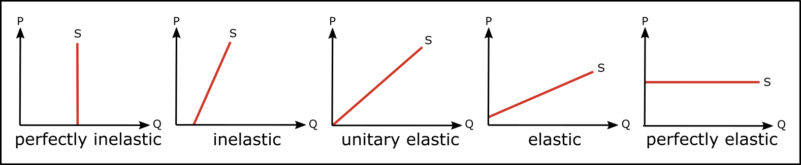
When the price elasticity of supply of a given good is high (i.e., that means that the general availability of the product is more likely to change whenever prices change), as the price of the good drops, producers generally begin producing less supply. Think about this:

When the price elasticity of supply for a given good is greater than unity, that means that the percentage change in the quantity supplied is greater than the percentage change in price. That is,

% change in Q_s > the % change in P

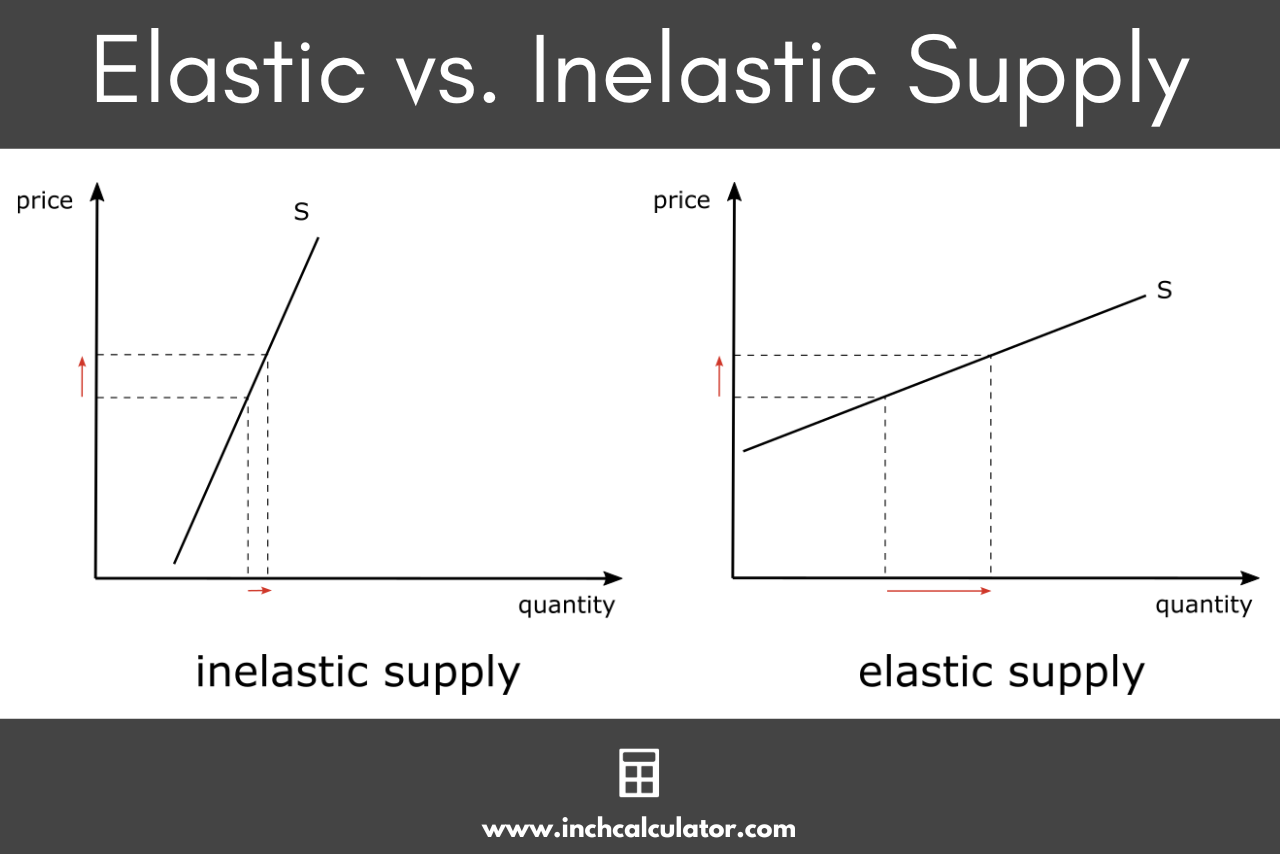
When the price elasticity of supply is low, or inelastic, that means that general changes in price are unlikely to influence the quantity of the good produced. That is,

% change in Q_s < the % change in P

This can occur when there is a long lead time to produce the good. For example, one cannot quickly build new electricity generation plants in response to an increase in demand for electricity. Due to regulatory factors (in particular) it takes many years to add new generation capacity.

Price Elasticity of Supply Formula

In order to calculate the price elasticity of supply (PES), you’ll need to know the original price, the final price, the original quantity, and the final quantity. Once you have determined these variables, you can then use the following formula:

PES = % change in quantity supplied / % change in price

% change in quantity supplied = Q₁ – Q₀ / (Q₁ + Q₀) ÷ 2 × 100

% change in price = P₁ – P₀ / (P₁ + P₀) ÷ 2 × 100

Suppose that the current price of a given unit is $20 and the product has an original supply of 100 units. Eventually, the price of the product increases to $25 and the supply of that product simultaneously increases to 150 units.

In this particular example, the price would have changed by 11.1% and the quantity being supplied would have changed by 20%.

To calculate the price elasticity of supply, simply divide 20% by 11.1%, which in this case would equal 1.8. In this case, the product would be considered somewhat elastic because the percentage change in quantity supplied was greater than the percentage change in price.

The Importance and Implications of the Price Elasticity of Supply

Let’s say that you are a used car salesman, and you are required to collect sales tax on every car that you sell. Who pays the sales tax?

Of course, the seller would prefer to pass the entire burden of the tax onto the buyer – but does this actually happen?

The answer is: no – it depends upon the elasticities of demand and supply. Of course, the seller would prefer to pass the entire burden of the tax onto the buyer.

For convenience, we will display the supply and demand “curves” in a way to indicate that one is more elastic – in this case the demand “curve” since used cars are not really necessities.

When any tax is imposed, it is imposed upon the seller to collect the tax and then remit it to the taxing agent (in this case, the Government, or G).

Clearly, the seller would like to pass on as much of the tax that he/she can to the buyer, so that the seller reduces his/her tax burden.

So, the following situation transpires:

Before the imposition of the tax, the market price of the vehicle was $7,000 (i.e., where supply and demand intersect) and the quantity of used cars sold was 750 million.

When the $1,000 tax is imposed on the seller, the supply curve shifts to the left (S + t), and the new market price is $7,400 and quantity is 500 million:

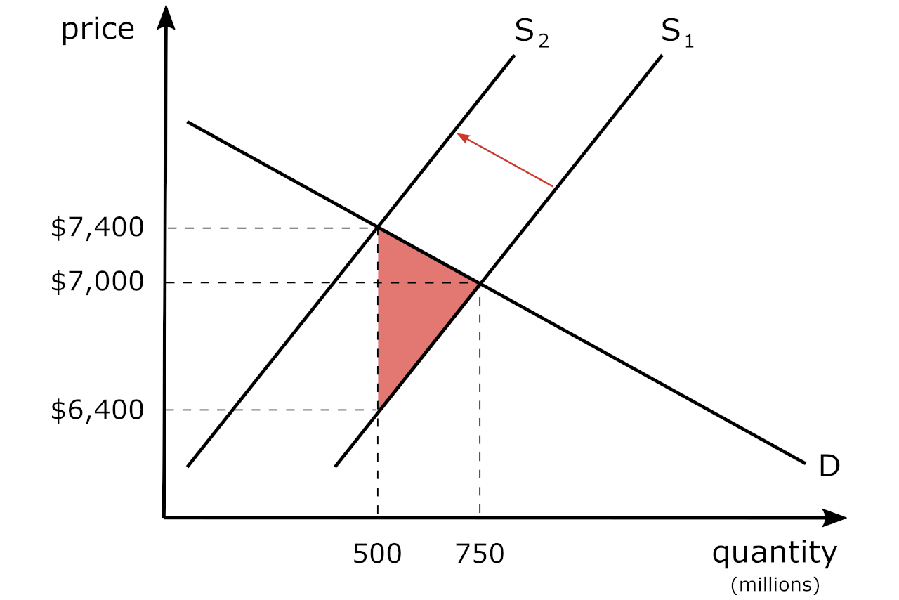
Several things are noteworthy:

1. Since the elasticity of demand is “more elastic” than that of supply, the seller bears more of the burden of the tax ($600 vs $400 for the buyer). Per the calculator, the PES = 4.5 while that of demand is -7.2.

2. In addition, the imposition of the tax creates a dead-weight loss; these are the transactions that would have occurred absent the tax (i.e., the sale/purchase of 250 million used cars at a price of $7,000 each). This is the area shaded in red in the chart above.

There are other extremes as well, for example, when supply is constrained, so that it is perfectly inelastic. This is displayed in the graph below.

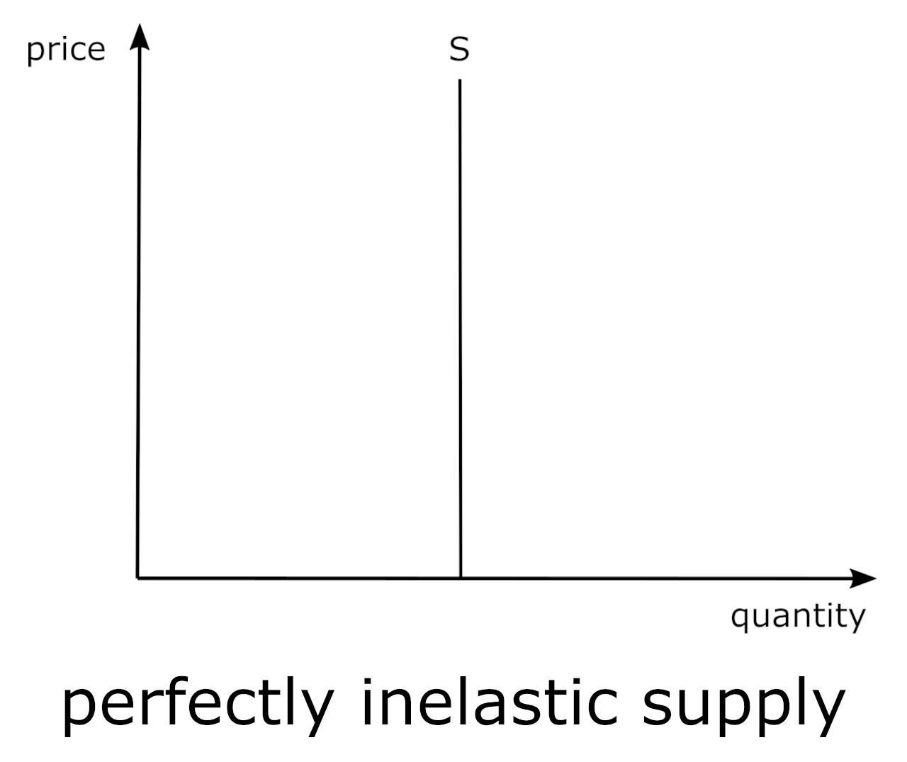
For example, in the short-term, the supply of crops such as grain or corn are constrained to the amount planted in the spring. There will be a limited harvest in the fall, regardless of the price.

Over the long-term, more crops will be planted as the prices rise, but some items are perfectly inelastic over the long-term as well, such as rare art or antiquities.

You might also be interested in our cross-price elasticity calculator.